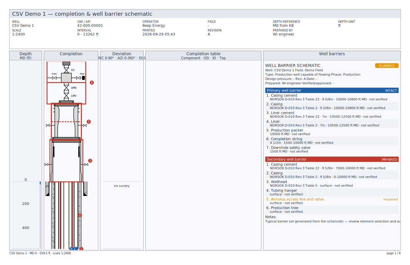
Reading the views
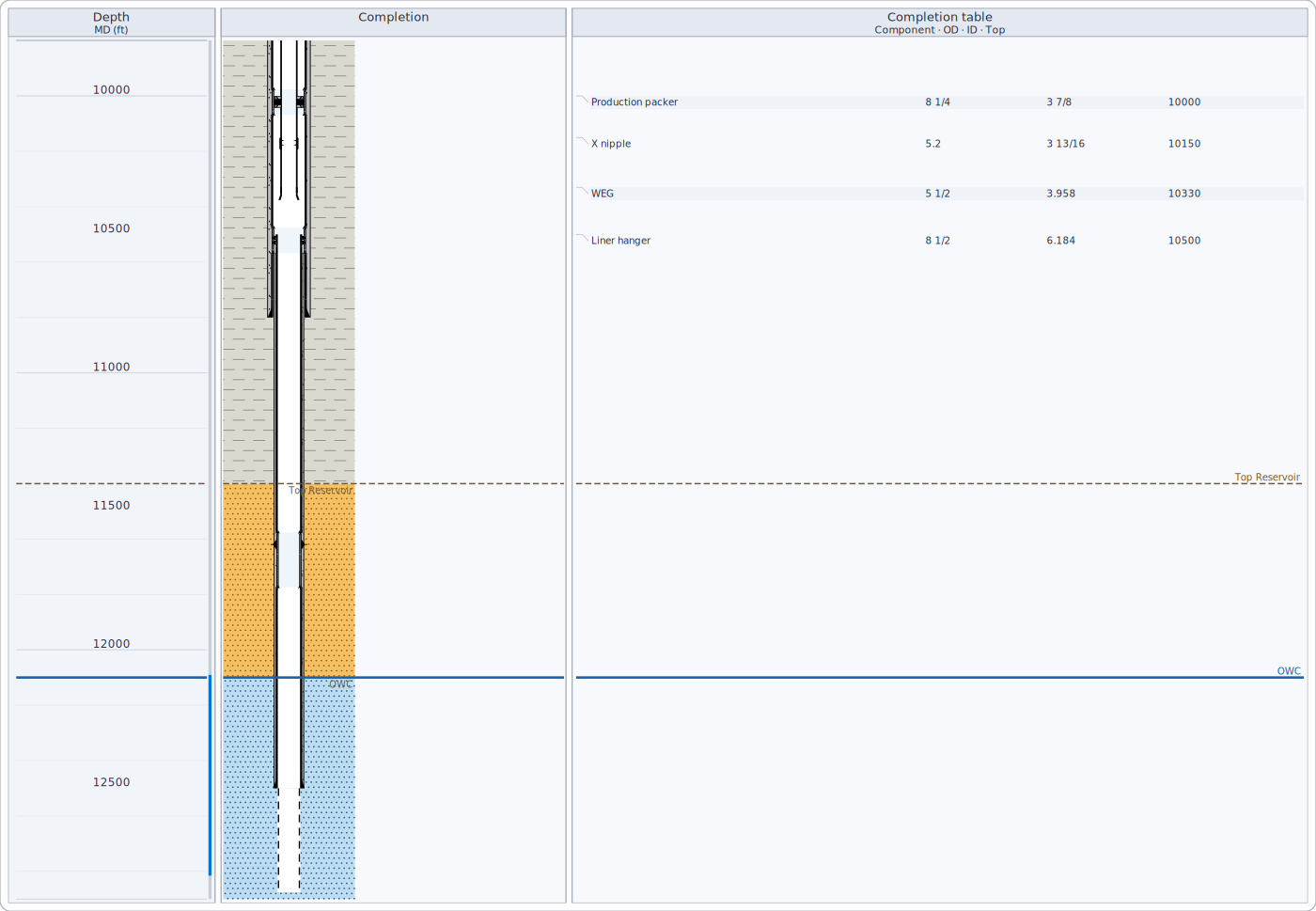
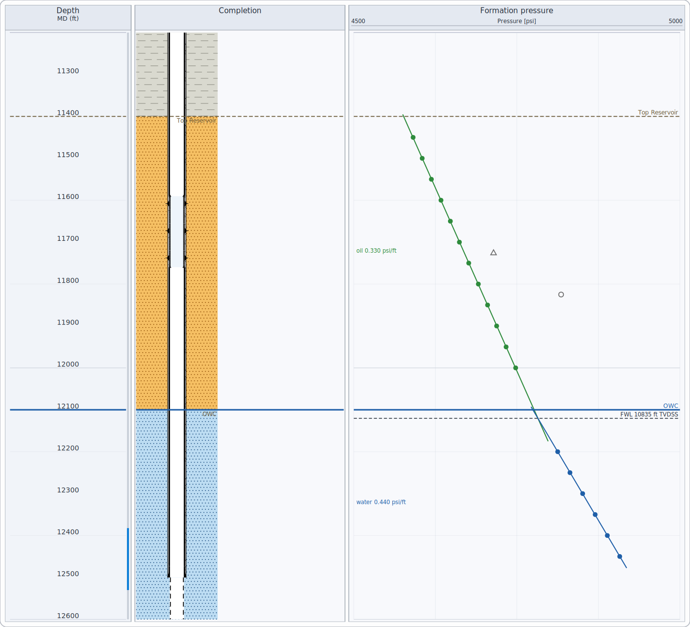
All depth-indexed views share one depth axis. The depth track states the reference (MD, TVD or TVDSS) and unit. A compressed depth scale gives more room to intervals with equipment and less to long empty casing; the axis labels stay true.
Completion schematic
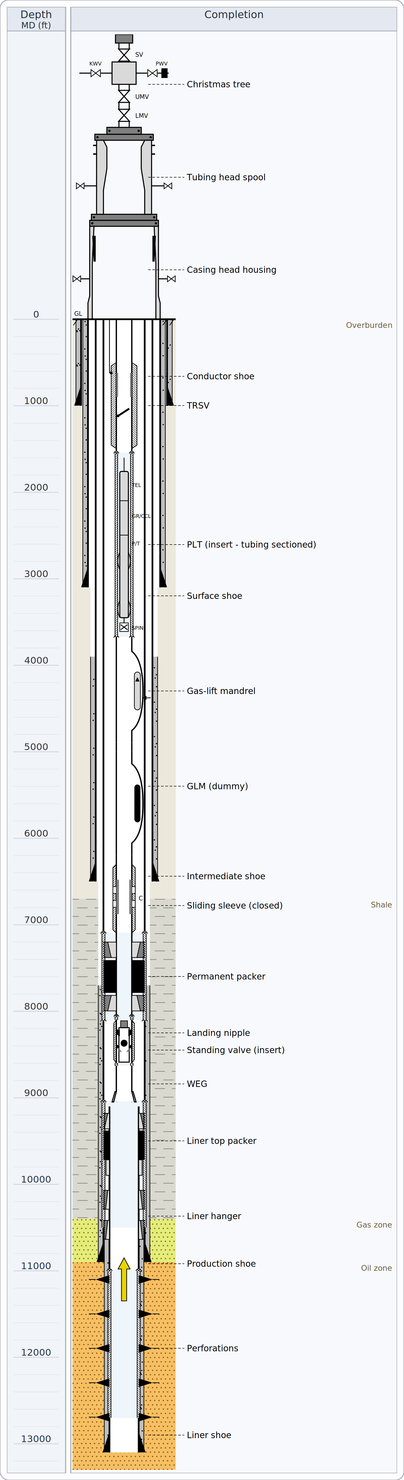
- Strings are drawn largest first: cement fills out to the hole wall, steel to the outside diameter, the bore to the inside. In scaled drawings diameters are true to each other and the hole wall is the real bit size of the section.
- Open hole below the deepest shoe is dashed at its bit size.
- The tally lists every item with depth, dimensions and provenance; the casing program lists strings with hole size, OD, ID, weight, grade, connection and top of cement.
Well logs
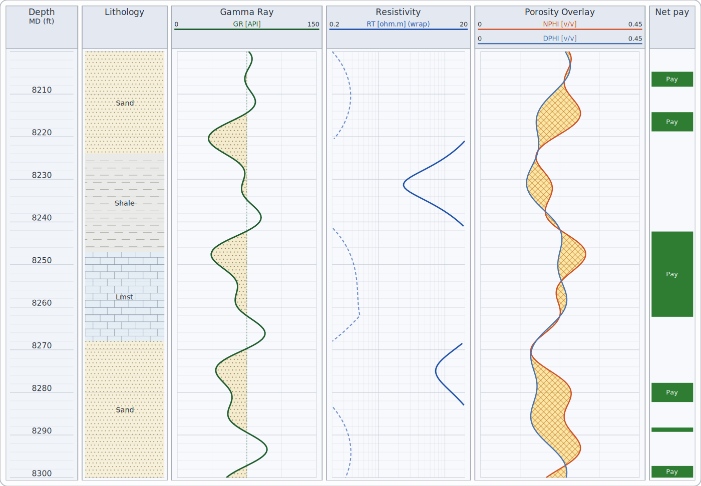
- Each curve's scale is drawn in its track header. Curves leaving their scale wrap to a backup scale when configured.
- Cutoff shading fills exactly where a curve crosses its cutoff.
- Curve families (gamma ray, resistivity, porosity, sonic, caliper...) and their colours and scales follow your environment's rules; resistivity is logarithmic by convention.
Computed curves
Shale volume (with the gamma ray), porosity (with the other porosity curves) and water saturation with bulk volume water (a Saturation track) can be computed from the logs; the methods and parameters are listed under Methods, standards & assumptions.
Notes and highlights
Add notes (a flagged text at a depth), arrows and highlighted intervals (a coloured band, for example over a pay zone) to a view - in one track or across all tracks. They are saved with the view, printed and exported with it, record who added them and when, and can be moved by dragging (when annotation editing is on) and undone. A note that points to a track you removed, or lies outside the depth range, is listed in the validation messages (WB030, WB031).
Editing the schematic
When editing is switched on, drag a packer, valve or other equipment to a new depth, or drag a casing shoe or cement top; every change can be undone. Equipment can also be added and removed. The edited schematic can be saved back to the well data: each value keeps its unit, and removed equipment is marked as removed rather than deleted, so the history is kept.
Depth matching and splicing
Curves from different runs can be matched in depth by dragging a selected curve up or down, or with tie points (a logged depth and the depth it belongs at; depths between tie points are stretched). Every shift is recorded - curve, tie points, reason, interpreter and date - and saved with the view, and can be undone. Two runs can be spliced into one curve at a chosen depth; the new curve's name records the splice.
Core data, dips and borehole images
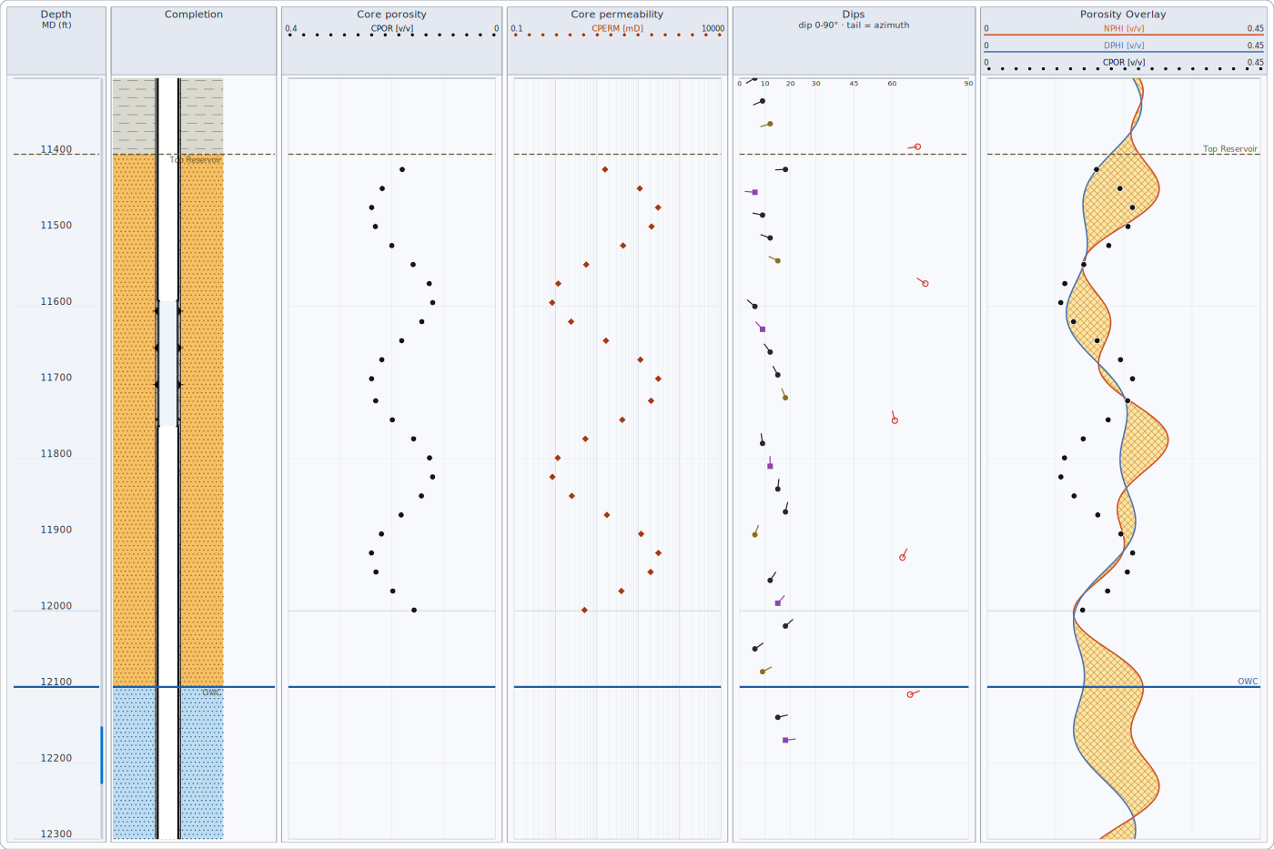
Dip tadpoles: position = dip angle, tail = dip direction (up is north). On borehole images a flat bed crossing the hole appears as a sine wave whose deepest point is on the down-dip side; picks are drawn as sinusoids.
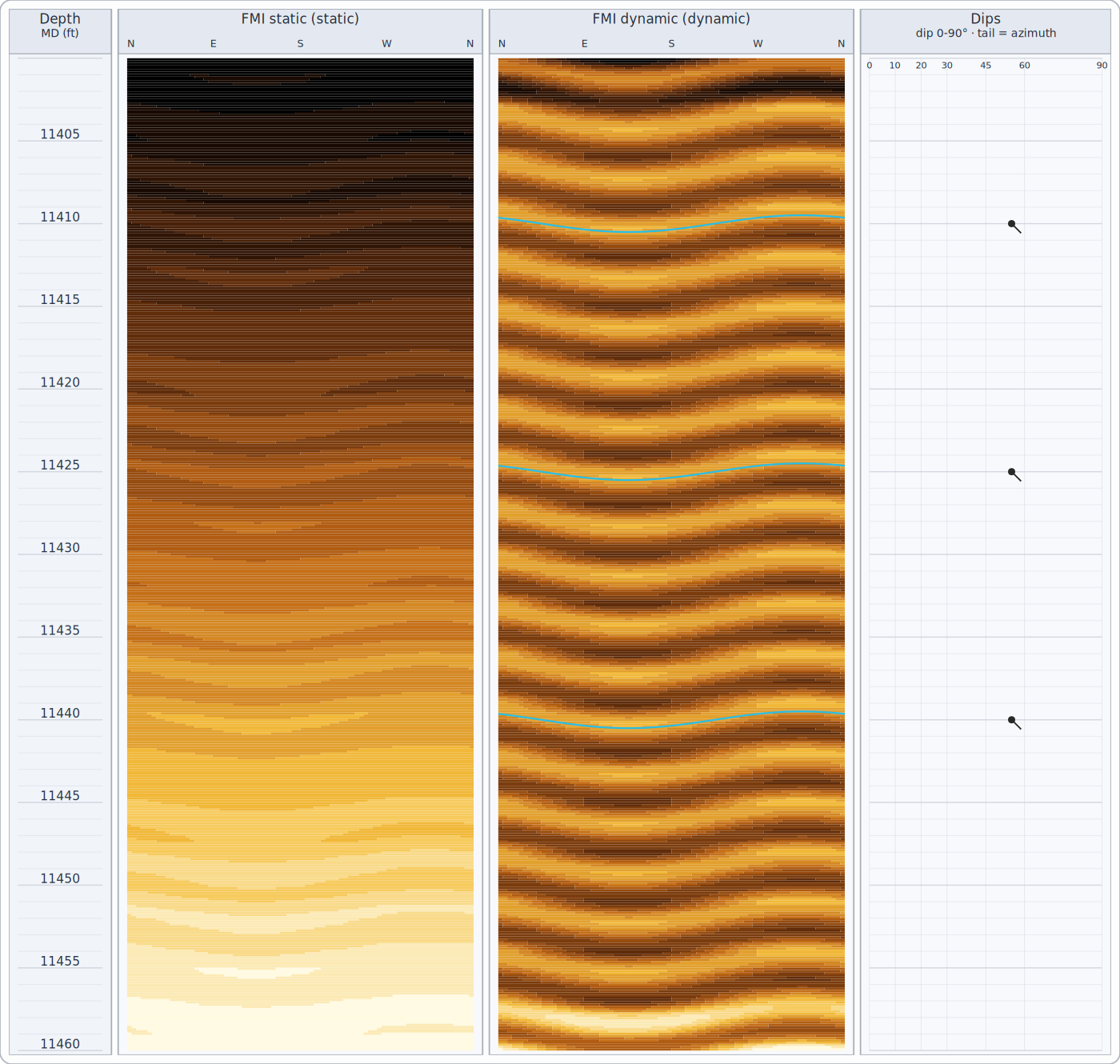
Static normalization scales the whole image at once and shows long trends; dynamic normalization rescales within a sliding depth window and brings out beds and fractures.
Cement bond
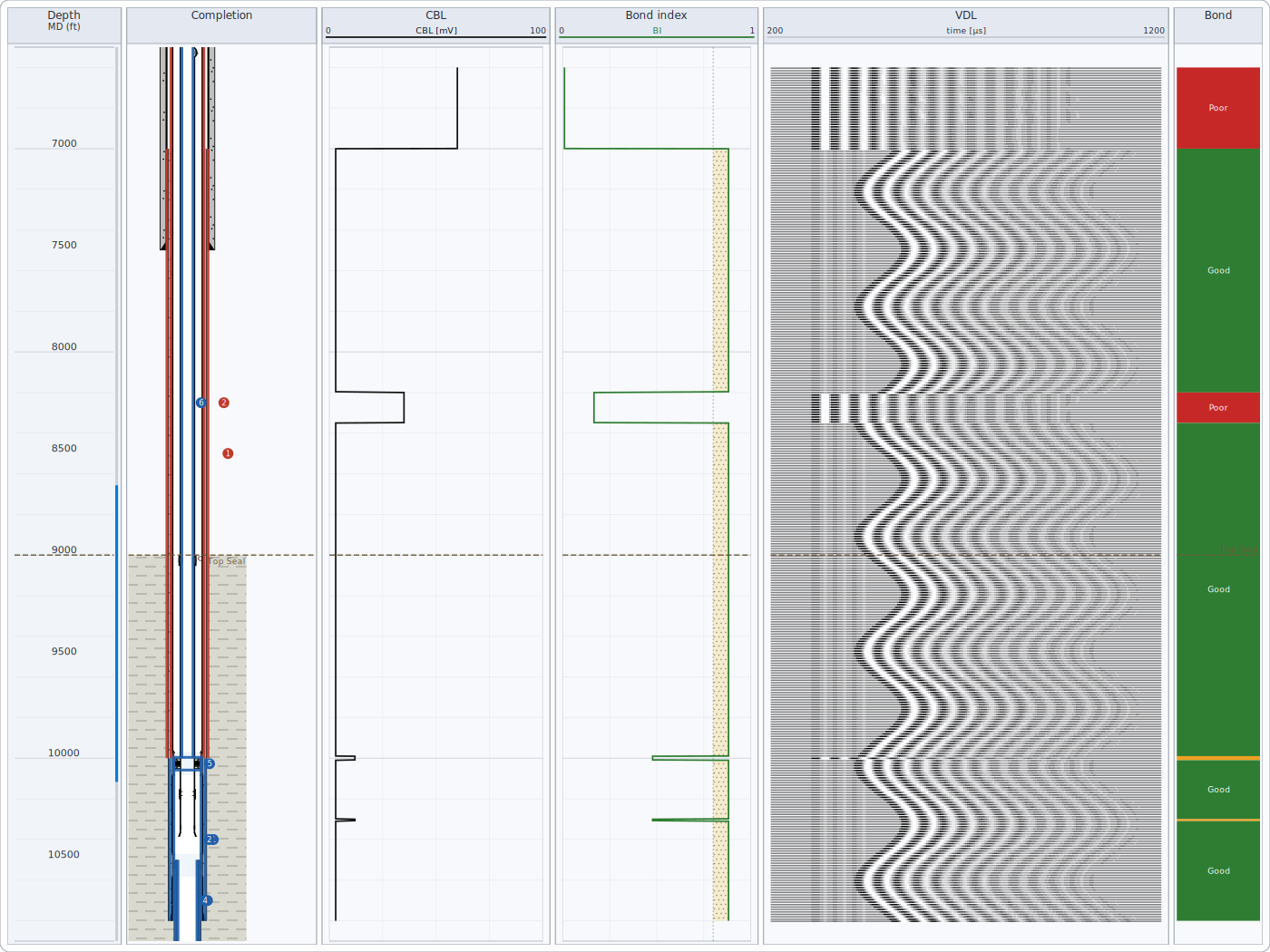
The bond index comes from the CBL amplitude between the free-pipe and fully-bonded calibration values set in your environment. Good bond over a sufficient continuous length can support a cement barrier element (see Well integrity).
Mud log
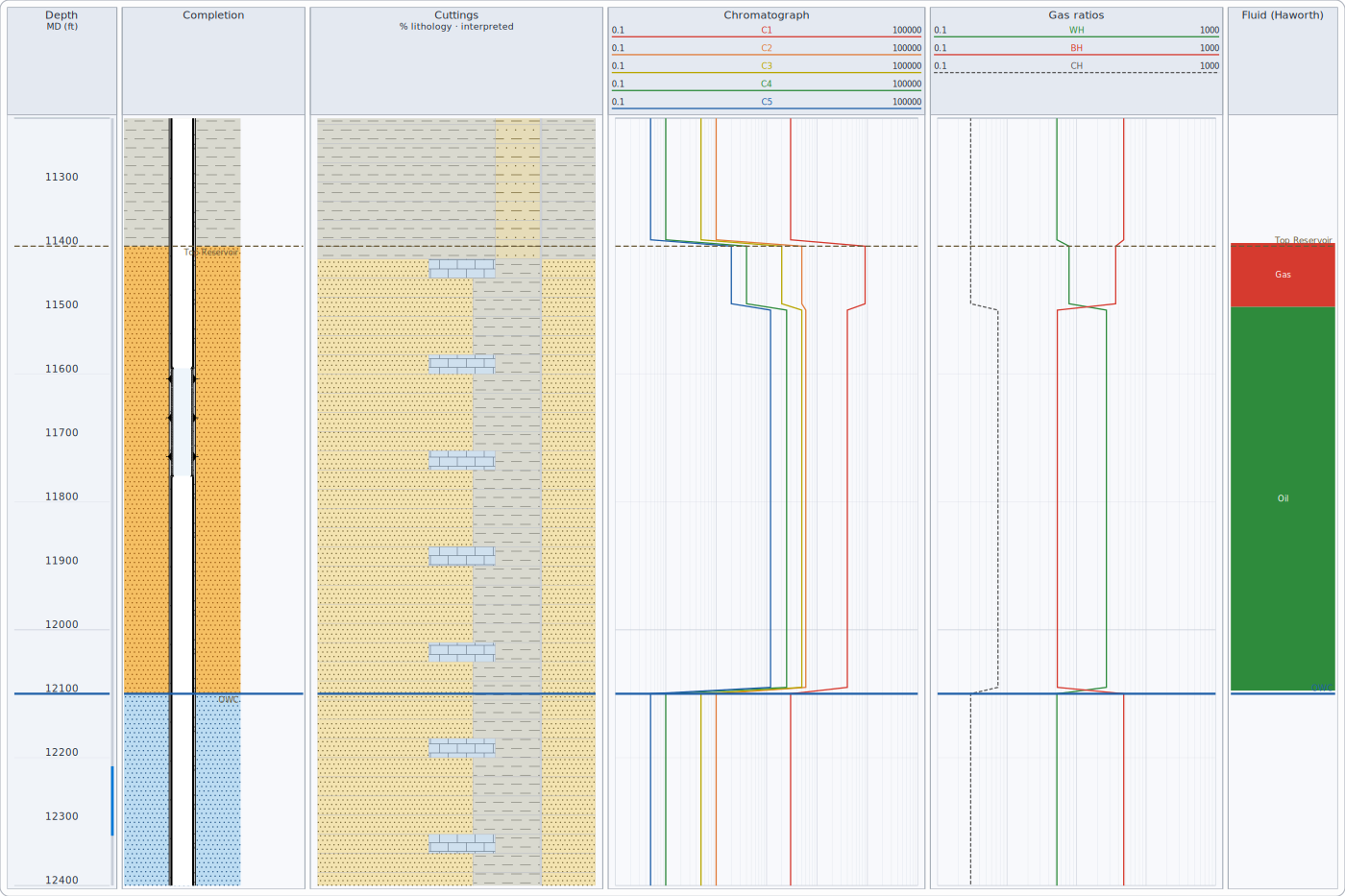
Fluid-character flags are shown only where total gas is a show above your threshold; background gas is not interpreted.
Well integrity
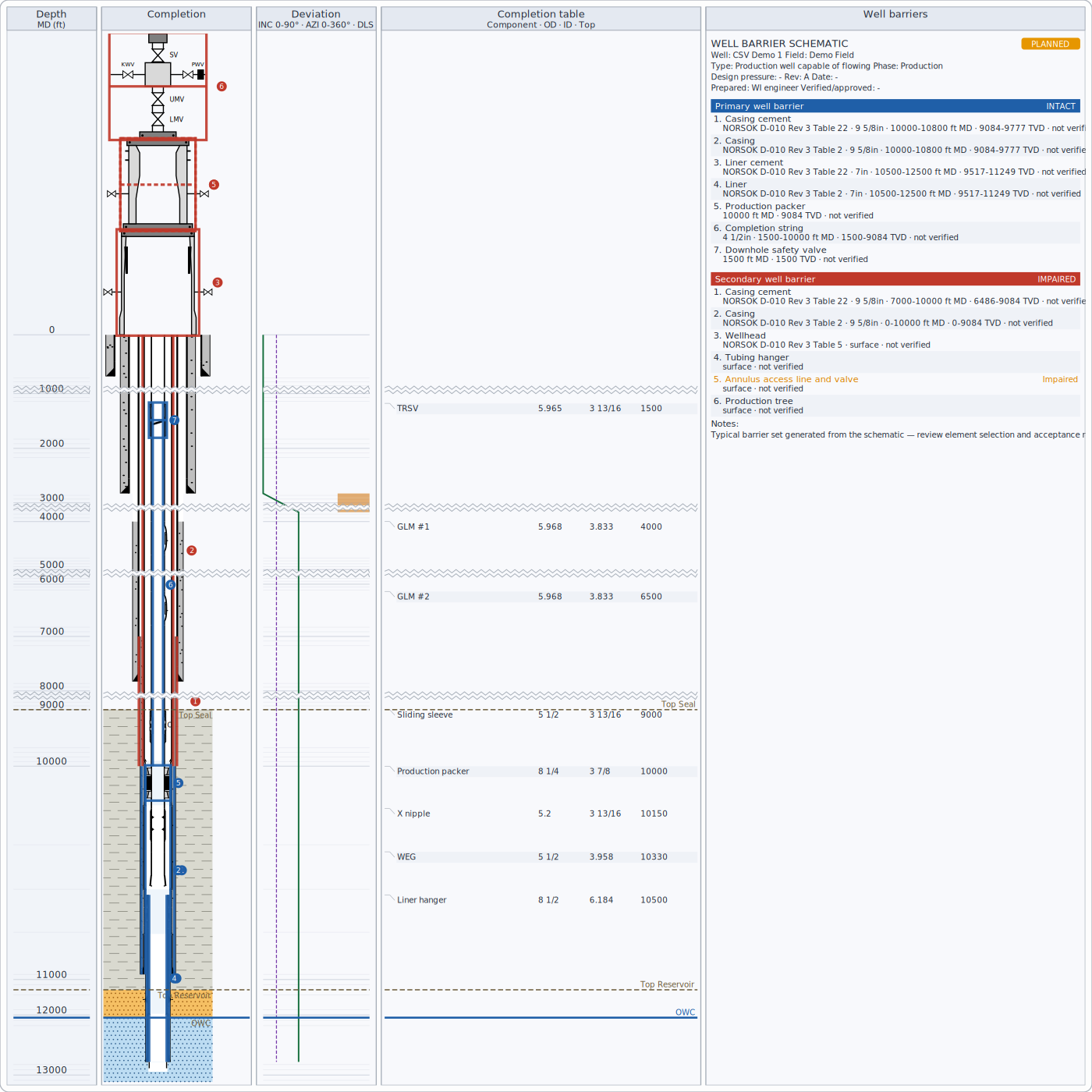
- Primary (blue) and secondary (red) envelopes follow the NORSOK D-010 convention; element status is shown by line style and in the table (intact, unverified, impaired, failed).
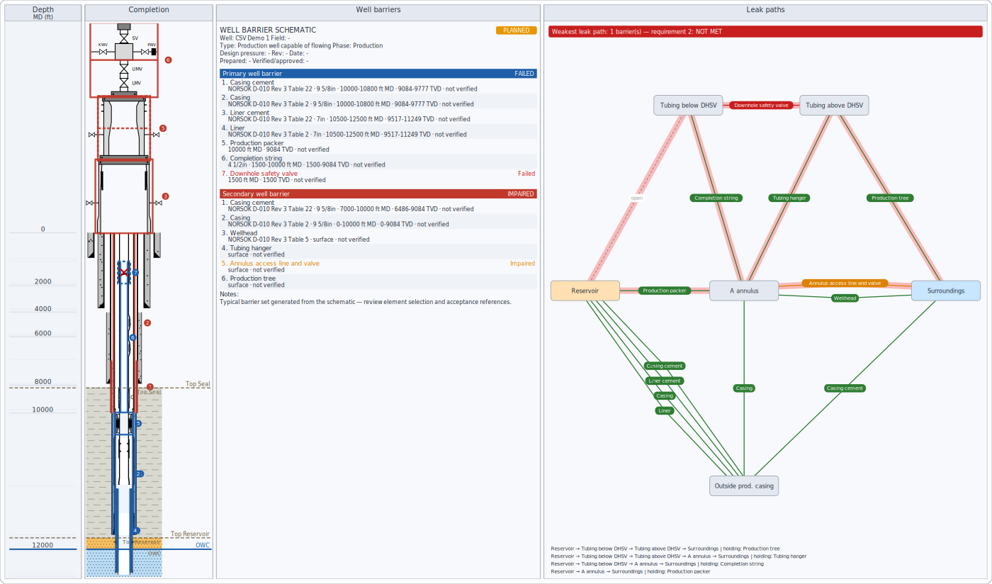
- Leak paths check every route from the reservoir to the surroundings and count the barriers still holding; the weakest paths are highlighted.
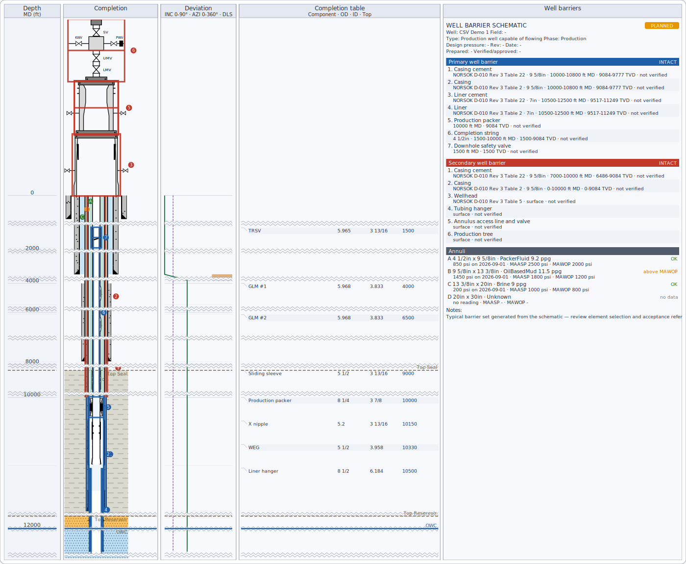
- Annuli (A, B, C...) show their fluids and pressure status against MAWOP and screening MAASP.
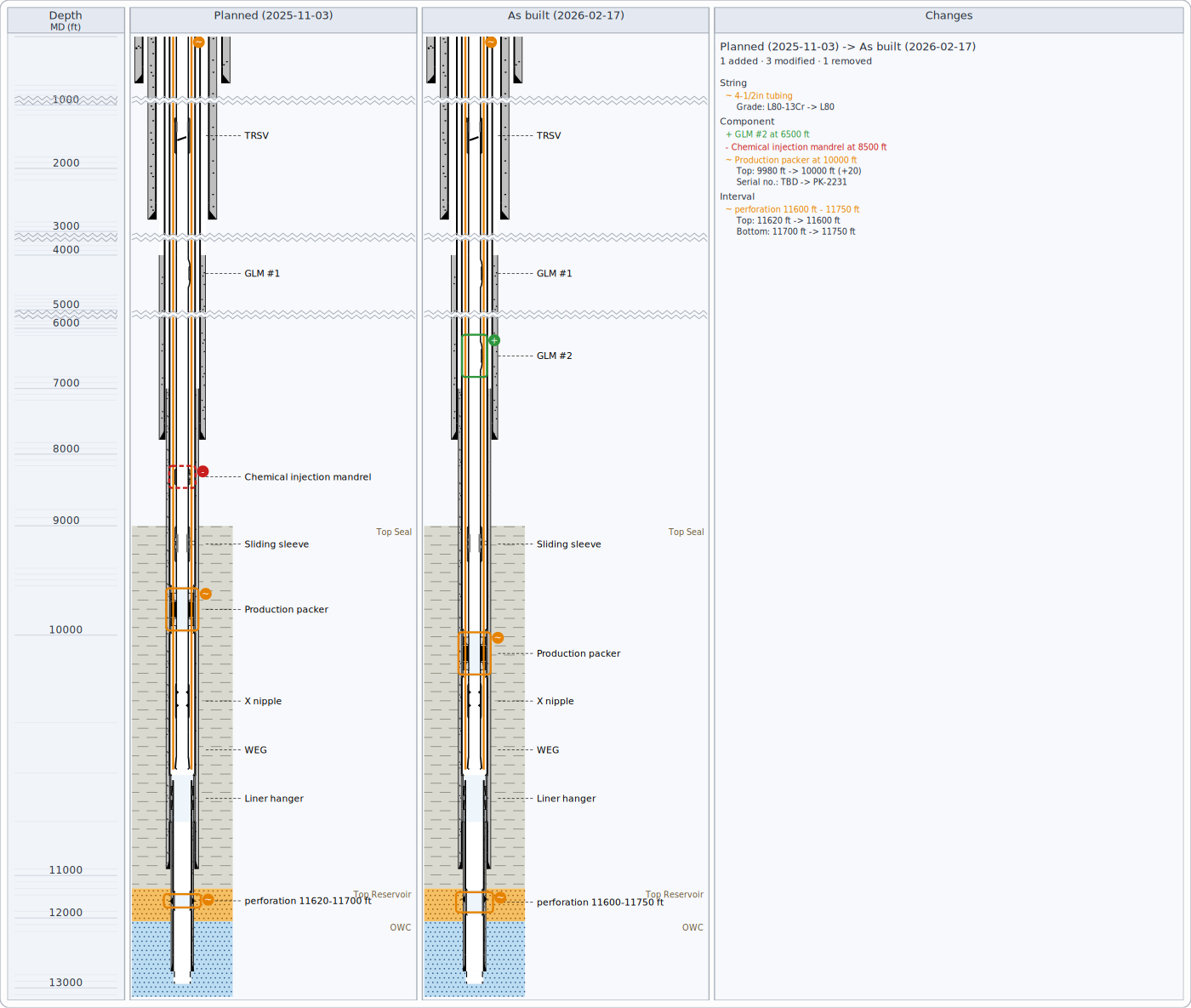
- Planned vs as built shows what was added, removed or changed.
- P&A checklist lists every abandonment requirement with a pass / fail mark and the details (plug depths and lengths, cement behind the plugs, sources of inflow); see Methods, standards & assumptions.
Keyboard and touch
| Well view | Key |
|---|---|
| Scroll a little / a screen | Up, Down / Page Up, Page Down |
| Go to the top / bottom | Home / End |
| Zoom in / out | + / - |
| Move the focus between tracks | Tab / Shift+Tab (the focused track has a dashed frame) |
| Undo / redo the last edit (tops, curve shifts, schematic, notes) | Ctrl+Z / Ctrl+Y |
| Delete the selected note (when note editing is on) | Delete |
| Clear the selection, stop shifting a curve | Escape |
On the map, the arrows move the map, + / - zoom, Home fits all wells, Tab selects the wells in turn and Escape stops drawing a section line. In a crossplot, Tab steps through the points in depth order and reads each one out. On a touch screen, pinch to zoom (the depth or map point under your fingers stays put) and drag with two fingers to scroll. Screen readers announce what each view shows - the well, the depth range, the focused track and the selection.
Crossplots
A crossplot shows two logs against each other, one point per depth: density against neutron (to read lithology and porosity) or resistivity against porosity (Pickett, to read water saturation). Points are coloured by zone or by a third log; move the pointer over a point to see its depth, values and zone. The lines on the chart are explained under Methods, standards & assumptions.
Map
The map shows the wells from above: surface locations with names, and the path of each deviated well to total depth, at the same scale east-west and north-south, north up, with a grid, scale bar and north arrow. Drag to move the map, use the wheel to zoom, click a well to select it. To make a cross-section, switch to section drawing and drag a line across the wells: the cross-section along that line opens with the wells near it (how near is a setting).
Correlation and cross-sections
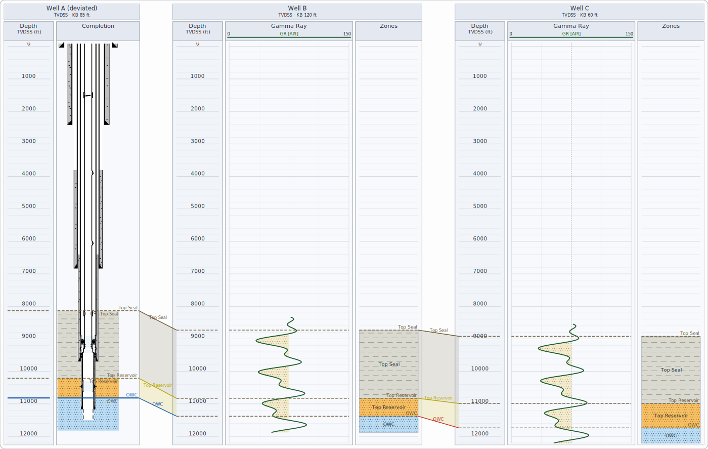
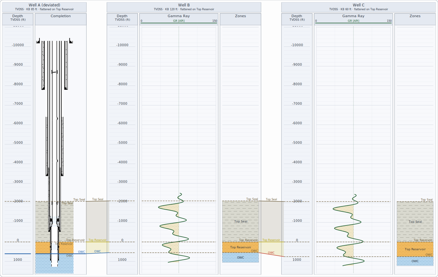
Tops are joined when they belong to the same unit - even when companies spell them differently, if your environment has a stratigraphic lexicon. Flattening on a top hangs every well from that top.
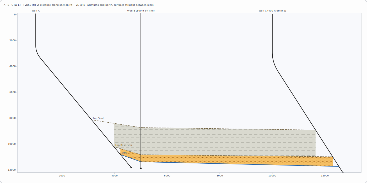
A cross-section places wells at their true horizontal distance along a map line and joins tops as surfaces.
Pinch-outs and truncations
When a formation top is found in one well but not in its neighbour, its surface ends between the two wells instead of stopping at the well. If a top above it is marked as an unconformity, the surface ends against it - the formation was eroded (truncation). Otherwise the formation thins out onto the surface below (pinch-out). Zones are filled down to the next surface present at each point, so there are no empty gaps. Surfaces can be drawn as straight lines between picks or as smooth curves that never go above or below the picks. Several sections can be shown one above another and printed together, one page each.
Well path
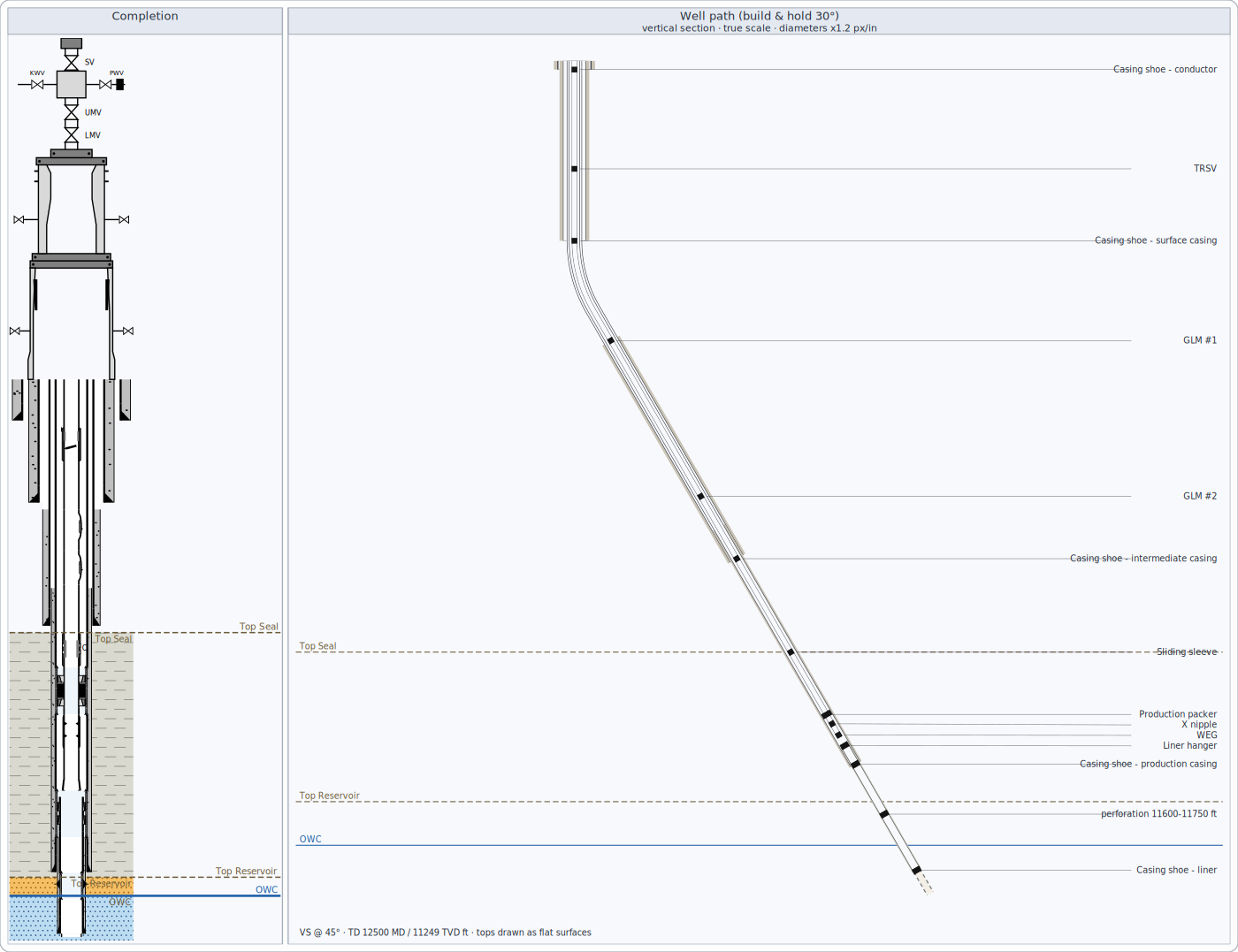
The path is drawn at true scale so build and hold angles look as they are; diameters are exaggerated (stated in the header).
Position uncertainty
The plan and section views can show ellipses around the well path: the area within which the well is expected to lie, at
two standard deviations by default. They are computed at each survey station from the survey's error sources and grow with
depth. The default error sources are a simplified set typical of MWD surveys, not a certified tool model: for anti-collision
or regulatory work, enter the error model of the survey tool actually used (survey.uncertainty in the environment).
Formation pressure
Printing
Printouts use an exact depth scale (for example 1:500), a header block with well information and your company fields, and a legend built from the tracks shown.